¶ Filter-based models of suppression in retinal ganglion cells: comparison and generalization across species and stimuli
Neda Shahidi1,2,3, Fernando Rozenblit1,2, Mohammad H. Khani1,2, Helene M. Schreyer1,2, Matthias Mietsch4,5, Dario A. Protti6, Tim Gollisch1,2,7
- Department of Ophthalmology, University Medical Center Göttingen, Göttingen, Germany
- Bernstein Center for Computational Neuroscience Göttingen, Göttingen, Germany
- Cognitive Neuroscience Lab, German Primate Center, Göttingen, Germany
- Laboratory Animal Science Unit, German Primate Center, Göttingen, Germany
- German Center for Cardiovascular Research, Partner Site Göttingen, Göttingen, Germany
- School of Medical Sciences (Neuroscience), The University of Sydney, Sydney, NSW, Australia
- Cluster of Excellence “Multiscale Bioimaging: from Molecular Machines to Networks of Excitable Cells” (MBExC), University of Göttingen, Göttingen, Germany
¶ Abstract
The dichotomy of excitation and suppression is one of the canonical mechanisms explaining the complexity of the neural activity. Computational models of the interplay of excitation and suppression in single neurons aim at investigating how this interaction affects a neuron’s spiking responses and shapes, for example, the encoding of sensory stimuli. Here, we compare the performance of three filter-based stimulus-encoding models in predicting retinal ganglion cell responses recorded from axolotl, mouse, and marmoset retina to different types of temporally varying visual stimuli. Suppression in these models is implemented via subtractive or divisive interactions of stimulus filters or by a response-driven feedback module. For the majority of ganglion cells, the subtractive and divisive models perform similarly and outperform the feedback model as well as a linear-nonlinear (LN) model with no suppression. Comparison between the subtractive and the divisive model depended on cell type, species, and stimulus components, with the divisive model generalizing best across temporal stimulus frequencies and visual contrast and the subtractive model capturing in particular responses for slow temporal stimulus dynamics and for slow axolotl cells. Overall, we conclude that the divisive and subtractive models are well suited for capturing interactions of excitation and suppression in ganglion cells and emphasize different temporal regimes of these interactions.
¶ Introduction
Sensory systems dynamically encode stimuli with a wide range of temporal characteristics, reflecting the complexity of changing scenes and self-motion in the natural world. A crucial mechanism for shaping and supporting the encoding of dynamic stimuli is thought to lie in the interplay of excitation and suppression, with the latter encompassing inhibitory synaptic signals as well as cell-intrinsic negative feedback, as can be mediated by voltage-dependent conductances. A simple example for this interplay of excitation and suppression is the limitation of response duration, leading to markedly transient responses of cells in the retina1, the thalamic lateralgeniculate nucleus2, as well as in auditory3 and somatosensory4,5 systems in response to an abrupt change in the strength of a stimulus. In many cases this response transiency has been explained by suppressive inputs coming with a short delay relative to the excitatory input, resulting in a brief window of opportunity for elevated activity before suppression dominates.
Similarly, the context-dependence of stimulus encoding in the visual system, such as found by varying background illumination, contrast, stimulus size, or stimulus motion, has been captured by suppressive interactions that act as a divisive gain modification6–8.
Suppressive mechanisms may also allow creating dynamic variations of stimulus integration time, as demonstrated by a conductance-based encoding model of suppression9,10. This provides a long temporal window for integrating sensory inputs when the signal-to-noise ratio is low allowing a neuron to average out noise and generate a robust response. A short integration window, on the other hand, enables the neuron to lock its response to the fast fluctuation of the sensory input.
To understand the role of the excitation–suppression interplay in generating various response dynamics, several filter-based encoding models have been proposed. The canonical idea behind these groups of models is to capture properties of excitatory and suppressive signals in independent temporal filters, whose signals are then combined to yield the activity of the modeled neuron. Here we focus on three classes of these models that have been proposed to capture the temporal response properties of the retinal ganglion cell (RGC) responses, using subtractive inhibition11, divisive suppression1, and activity-dependent negative feedback10,12,13, respectively. For the subtractive and the divisive models, the suppression is derived in a feedforward way by applying a filter to the same input signal that feeds the excitation. For the feedback model, on the other hand, suppression is triggered by the spikes that are stochastically generated by the model cell and that provide the input to the suppressive filter.
To maximize the similarity between the training algorithms and optimization constraints across the different models, we trained and tested the three suppressive models as well as a feedforward linear-nonlinear (LN) model within a unified computational structure, where each of the models could be implemented by fixing certain model parameters to specific values. We applied this framework to RGC responses recorded from retinas of axolotl, mouse, and common marmoset under stimulation with full-field white-noise flicker of light intensity. The unified implementation and datasets allowed us to compare the models directly and to identify the cell and stimulus types for which each model outperforms the others.
One of the main challenges for developing encoding models is their generalization to different classes of stimuli. While we train the models on data from white-noise stimuli, as is customarily done for these and comparable models, we here also test the performance of the suppressive models on stimuli that contain sinusoidal frequency and contrast sweeps. The ability of a model to generalize to such non-stationary stimuli helps provide an understanding of how the model captures retinal stimulus processing in a complex setting with varying stimulus statistics.
¶ Results
¶ Comparison of three suppression models in a unified framework
We implemented three filter-based neuron models of suppression, based on subtractive, divisive, and feedback interactions, respectively, as well as an LN model in a unified structure (see Methods; Fig. S1). This common computational framework aimed at maximizing similarities in the models’ motifs as well as in training and testing procedures. In this framework, each model yields an integrated signal that encompasses the effects of excitation and suppression and that—after nonlinear rectification—is used for the generation of time-varying spike counts in small discrete time windows using a Poisson random process. What differs between the models is how the integrated signal is obtained (Fig. 1A). The subtractive and divisive models each had two upstream branches, each with its own stimulus filter and subsequent nonlinear transformation. The two branches were then combined by a subtractive or divisive operation, respectively. The upstream filters were unconstrained, whereas the shapes of the nonlinear transformations were constrained to support the excitatory or suppressive action: The nonlinearities for the excitatory and suppressive branches of the subtractive model as well as for the excitatory branch of the divisive model were required to be monotonically increasing, whereas the suppressive branch of the divisive model had a nonlinearity that was “bump-shaped”, i.e., monotonically increasing on the side of negative inputs and monotonically decreasing on the positive side. The feedback model and the LN model each had a single (excitatory) upstream branch for stimulus filtering and nonlinearly transforming the filtered signal into a firing rate. For the feedback model, an additional filter is applied to the model-generated spikes, and the upstream and feedback filter signals are then summed. Note that both the feedback and the LN model have an additional nonlinearity just prior to the stochastic spike generation, the nonlinearity prior to spike generation that is common in all models. For the LN model, this means two successive nonlinear stages that together constitute the typical single output nonlinearity of this model. That this is here subdivided into two stages is a concession to the unified structure of all models. For training, the models, the filters, and the nonlinearities were parametrized using sets of basis-functions (see Methods). The output rectifier was parametrized using a softplus function (see Methods). All models were trained using a maximum-likelihood approach with a block-coordinate ascent algorithm, in which we iterated the sequential update of each block of the model (a filter or a nonlinearity) to maximize the likelihood function while other blocks were kept constant (see Methods).
The models were trained and tested on ganglion cells recorded from retinas of axolotls (n = 15 recordings), mice (n = 8), and marmosets (n = 10). Spikes were recorded with multi-electrode arrays while the retinas were stimulated using full-field Gaussian white noise. For axolotl and mouse, the stimulus consisted of an alternating sequence of 30 s (axolotl) or 15 s (mouse) of nonrepeating white noise, which was used for training the models, and 10 s (axolotl) or 5 s (mouse) of “frozen noise”, i.e., a fixed white-noise sequence that was presented repeatedly, which we heldout for testing. In the marmoset data, no frozen-noise stimulus was used. Therefore, we trained using 15 s segments interleaved with 5 s held-out testing segments. The model performance was assessed by calculating the average information provided by the model for each spike2,14, assessed on the held-out testing data segments. Note that this measure of model performance does not require repeated trials.
Our analysis included 607 axolotl, 335 mouse, and 370 marmoset cells that responded reliably to the white-noise stimulation. ON-OFF cells, i.e., cells that respond to both step-wise increases and decreases in light intensity, were removed because their responses cannot be captured using the monotonically increasing excitatory nonlinearities, as applied in all four models. Comparing the performance of the three suppressive models to that of the LN model showed that each of the suppressive models predicted responses better than the LN model for the majority of cells (subtractive: 97%, divisive: 96%, feedback: 85%). To quantify for each cell and each suppressive model how much predictive power was gained by the addition of the considered suppressive component, we computed the excess performance as the difference between the model performance of the considered suppressive model and that of the LN model. For this comparison, we selected the LN model that was fitted via the unified structure of Fig. S1 because, for almost all cells, this fitted LN model performed equally or better than alternative LN models for which the stimulus filter was either obtained as the spike-triggered average or the first principal component obtained from a spike-triggered-covariance analysis (Fig. S2). Nevertheless, suppressive models generally outperformed the LN model, and the excess performance of the bestperforming suppressive model for 95% of the cells was in the range of [0.03, 0.94] bits/spike for axolotl, [0.01, 0.29] for mouse, and [0.001, 0.23] for marmoset. The best-performing model was the subtractive model for 46%, the divisive model for 42%, and the feedback model for 12% of the cells.
For recordings from axolotl and mouse retina, visual stimulation included repeatedly inserted sections of the same (randomly generated) stimulus sequence (“frozen noise”). These sections, which were not used for parameter fitting, allow measuring a firing-rate profile. Comparison with model-predicted firing rates then provided a measure of explained variance (Fig. S3). This yielded qualitatively similar findings as the evaluation via per-spike information (Fig. 1B,C). In particular, the explained variance was generally higher for all suppressive models than for the LN model (p << 0.001), and the excess performance, as obtained by subtracting the explained variance of the LN model from that of the considered subtractive model, was more pronounced for the subtractive and the divisive model as compared to the feedback model.
¶ Cell-type specific comparison of subtractive and divisive model
As the subtractive and divisive models generally had the top performance among the four assessed models, we compared the performance of these two models more closely and aimed at determining for which cells one or the other of these two models was superior. Comparing the performances on a cell-by-cell basis (Fig. 2A) indicated that, in the axolotl retina, there is a group of cells for which the subtractive model outperformed the divisive model. For the rest of the axolotl cells as well as for mouse and marmoset cells, the performances of the two models were comparable, with the divisive model performing slightly better (p < 0.003; Wilcoxon signed rank test with false discovery rate for multiple comparison correction15; Fig 2A).
To understand the diversity of the cells in the axolotl retina, we classified them into ON and OFF cells as well as into slow and fast cells. To do so, we computed the temporal filter for each cell as the spike-triggered average under the temporal white-noise stimulation and clustered cells in the space of the first two principal components of all filters (Fig. S4). Based on this classification, we found that the relative performance of the subtractive and the divisive model depended on the kinetics of the considered cell. For fast cells, the difference between the performance of the subtractive and the divisive model was small, with the subtractive model just slightly better (fast OFF: mean difference = 0.026 bits/spike, p = 0.005, fast ON: mean difference = 0.02 bits/spike, p = 0.7). For slow ON and slow OFF cells, on the other hand, the subtractive model performed substantially better than the divisive model (slow OFF: mean difference = 0.08 bits/spike, p << 0.0001, slow ON: mean difference = 0.1 bits/spike, p << 0.0001; Fig 2B).
To better understand how the suppressive components of the subtractive and the divisive model help improve over the LN model, we examined the model components for individual sample cells more closely. For the sample axolotl slow OFF cell in Fig. 3A, the subtractive and the divisive model yielded qualitatively similar stimulus filters for both the excitatory and the suppressive model branch. However, the upstream suppressive functions of the subtractive and divisive models were substantially different for this cell in that the suppression of the subtractive model allows a gradual decline of suppression as the activation of the suppressive filter becomes more negative (Fig. 3Aii), whereas the divisive model had only unilateral, rectified suppression with essentially no sensitivity of the suppressive component to filter activations near or smaller than zero. Therefore, the subtractive model captured the fluctuations in the response of the cell while the divisive model, to a lesser degree, and the LN model, to a greater degree, generated stretches of near-flat outputs with little modulation for this cell.
For the mouse cell in Fig. 3B, the fast-OFF cell in Fig. 3C and the marmoset cell in Fig. 3D, the suppressive filter for the divisive model resembled the excitatory filter, except for a shift to the right. That resulted in a suppressive response that came with a slight delay compared to the excitatory response, leading to a timelier prediction of the falling edge of a firing-rate response peak compared to the LN model. Across all recorded cells 57% of axolotl cells, 79% of mouse cells and 70% of marmoset cells had suppressive filters that lagged the associated excitatory filters by 1-2 stimulus frames (~30-60 ms for axolotl; ~16-33 ms for mouse and marmoset; Fig. 3E). Also for 57% of the axolotl cells, 90% of the mouse cells, and 88% of the marmoset cells, the divisive nonlinearity was symmetric (Fig. 3F; asymmetry index < 0.5) meaning that flipping the suppressive filter upside down should yield a similar suppressive signal.
The subtractive model for these three cells, on the other hand, yielded a diverse set of excitatory and suppressive filters. Across all recorded cells, 40% of axolotl cells, 12% of mouse cells and 5% of marmoset cells had suppressive filters lagging the excitatory filters by 1-2 stimulus frames while 32% of axolotl cells, 23% of the mouse cells and 28% of the marmoset cells had suppressive filters leading the excitatory filter by 1-3 stimulus frames (Fig. 3G). Yet, model performance was generally similar to the divisive model, suggesting that different computational motives might converge to inherently different, but equally good solutions.
¶ Differences in model performance between sustained and transient cells
Delayed suppression that comes with a similar stimulus dependence as excitation is a proposed mechanism for generating sharp transient responses1,2. The delayed suppression may result, for example, from feedforward inhibition with additional synaptic transmission delays as compared to excitation, which generates a brief window for excitation to elicit spikes before the suppressive component terminates the response.
Effects of suppression on the transiency of responses are most easily assessed for strong sudden increases in stimulus strength. For a subset of marmoset cells which had also been stimulated using full-field steps in light intensity (100% contrast), we therefore assessed how much suppressive components helped predict responses to the Gaussian noise, and how that related to the transiency of the response to light-intensity steps. Cells were classified as either transient or sustained by comparing the strength of the initial response peak to the sustained activity beyond 300 ms after stimulus onset (Fig. 4A). For the sample session of Fig. 4B, the excess performance of suppression (from the best performing suppressive model for each cell) was significantly larger for the transient-ON cells compared to the sustained-ON cells, suggesting a weaker suppression in the sustained-ON cells. 4 out of 6 sessions showed a similar difference between the transient and sustained-ON cells (Fig. 4C). Comparing the ON cells to OFF cells, on the other hand, did not reveal a systematic difference in the excess performance (Fig. S5). This indicated that, indeed, explicit suppressive model components help explain the response brevity of transient ganglion cells.
¶ Generalization to stimuli with varying contrast and temporal frequency
The presented findings so far were mostly based on the performance of the suppressive models on white-noise stimuli. Thus, an important question is how the derived models generalize to stimuli with different, non-stationary statistics, such as variations in contrast or temporal frequency. For a subset of recordings from marmoset cells, we had applied a full-field chirp stimulus16, which contained two sections of sinusoidal light-intensity modulations, one with monotonically increasing contrast (“contrast sweep”, starting at 0% and ending at 100% contrast, duration of the sweep = 8 s, frequency = 4 Hz) and the other with increasing frequency at fixed contrast (“frequency sweep”, ramping up from 0 Hz to 15 Hz, duration of the sweep = 8 s, contrast = 100%). We therefore tested the performance of the models that were trained using the white-noise stimulus on the cells’ responses to these sinusoidal light-intensity modulations.
As illustrated by the model responses for two sample cells shown in Fig. 5A-D, the degree to which the prediction of each model matched a cell’s response varied with the frequency and contrast of the stimulus. We quantified this effect for the contrast sweep stimulus by calculating the explained variance (R2) for each model within a sliding window of 150 ms duration, shifted along the time course of the stimulus at steps of 16.7 ms (1 stimulus frame). For this marmoset cell, the divisive model outperformed the others for any contrast higher than 34% (Fig. 5B). For each marmoset cell, we calculated the performance range as the range of contrasts for which R2 > 0. The performance range was significantly larger for the divisive model, compared to other models (p << 0.0001; Fig. 5E), indicating that the divisive model generalized over a wider range of contrasts. This finding is consistent with a previous report1 that the divisive model captures the adaptation of ON-alpha ganglion cells of mouse to changes in contrast of a white-noise stimulus.
Similarly, we quantified the frequency-dependency of model performances using the frequency sweep stimulus. As shown in Fig. 5C for a second sample cell, the subtractive model outperformed the other models when the frequency of the stimulus was below 6 Hz, whereas the divisive model had the highest performance among the tested models for frequencies above 6 Hz (Fig. 5D). For each cell, we calculated the low-frequency performance, i.e., the average explained variance for first 317 ms of the frequency sweep (analysis window of 150 ms, shifted 10 times, each time 16.7 ms which was the length of a stimulus frame) as well as the performance range, i.e., the range of frequencies for which R2 > 0. For the subtractive model, the low-frequency performance was significantly higher than for the other models (p < 0.03; Fig. 5F, left), indicating that this model performed better in capturing the cells’ responses to low frequencies in the chirp stimulus. On the other hand, it was again the divisive model—like for the contrast sweep—that had the largest performance range (p < 0.004; Fig. 5F, right), indicating that this model generalized better over the frequency range of the chirp stimulus.
¶ Discussion
The interplay of excitation and suppression is a central theme of how nervous systems shape their responses to sensory stimuli. How to reflect the suppression in computational models of single cells is thus a question of broad interest. We here found that three different, previously introduced approaches to incorporate suppression into filter-based models can all be used to improve response predictions over the commonly applied single-filter model, the linear–nonlinear model. Moreover, the subtractive and the divisive model generally outperform the feedback model for most cells in axolotl, mouse, and marmoset.
The fact that the subtractive and the divisive model overall performed quite similarly for most cells might seem a bit disappointing at first glance, as the lack of a clear “winner” makes inference about the type of excitation–suppression interaction difficult. On the other hand, this null-result means that, from a phenomenological perspective, the details of how suppression is included in the model matters much less than having a suppressive component at all, indicating that different interactions can achieve similar functions by different means. The functional equivalence of different model structures is reminiscent of studies of the stomatogastric ganglion in lobster where the potential variable implementations of the same circuit function has been forcefully demonstrated17.
More detailed comparisons between these two models, however, revealed systematic differences in how performance depended on species and stimulus features. The subtractive model performed better for capturing responses of slow axolotl cells to white- noise stimuli and responses of marmoset cells to low-frequency parts of the chirp stimulus. The divisive model, on the other hand, displayed greater potential for generalizing over wider ranges of contrast and frequency. This suggests that different neural suppression mechanisms may dominate for different temporal scales of stimulation and response and that the two models differ in how well they capture the effects of these specific mechanisms. In particular, the subtractive model may particularly account for biological mechanisms that prevail in slow cells or that take effect when the stimulus is predominated by slow frequencies.
A technical aspect that may contribute to limiting the performance of the feedback model is the fact suppression in this model depends on the occurrence of spikes, which are sparse and stochastic in the model. This limits the effectiveness of the suppression mechanism (e.g., it cannot suppress a spiking event that is not preceded by another spiking event) and induces variability in the predicted responses. Alternative implementations might let the feedback depend on the continuous internal signal before spike generation18 or might apply a deterministic spike generation process13,19.
In the present study, implementation of the compared models was guided by the goal of a common framework that made the model structures and the training most comparable. Yet, the number of free parameters was not identical between all models. Given the complexity of the models, this raises the question whether the comparison might be influenced by over-fitting, which might reduce performance on the test data for models with a higher number of degrees of freedom. However, the subtractive and the divisive model actually had the same number of free parameters so the observed differences are unlikely to arise from differences in fitting accuracy. Additionally, the overall performance of these two models was higher than the feedback and the LN models which both had fewer free parameters. Therefore, we over-fitting is not likely to limit the interpretability of our findings.
A limitation of the present study is that we restricted our analysis to the use of full-field stimuli without any spatial structure. We made this choice in order to limit the number of free parameters in the model as well as to allow comparison between cell types and models independent of the how well the spatial filtering and potential nonlinearities in spatial stimulus integration20–23 are captured. On the downside, the use of full-field stimuli makes our analysis insensitive to the spatiotemporal structure of suppression, in particular by not providing for a dedicated suppressive signal pathway from the receptive-field surround.
A particular aspect of our study was the comparison of the models across ganglion cells from different species. This showed an overall high level of consistency of the findings; the similar performance of the subtractive and the divisive model and the generally lower performance of the feedback model was observed in salamander as well as mouse and marmoset. One someone exceptional group of cells was the set of slow axolotl cells that displayed a clear preference for the subtractive model over the divisive model. For these cells, the slowness is particularly pronounced, as filters and response kinetics in the axolotl are overall slower than in the other species, perhaps partly owing to the lower temperature at which the axolotl experiments were performed. This may make the subtractive model, which appeared to generally capture slow temporal dynamics better, particularly suited for the slow cells in this slow retina.
For marmoset ganglion cells, we found that including suppression in the response model, either through the subtractive or the divisive model, was more relevant for transient cells than for sustained cells, in particular when considering responses to steps in light intensity. In the primate retina, the ganglion cells types of midget and parasol cells numerically make up the majority of the RGC population24,25, and among these, parasol cells tend to have transient responses and midget cells sustained responses25–27. It thus seems likely that it is the parasol cells for which including suppression in the model is particularly relevant, though we have no independent classification of parasol and midget cells for the present datasets.
Like many other investigations of neuronal response models to sensory stimulation, we based our model fits on recordings under stimulation with white-noise signals. There is increasing awareness, however, that an important follow-up step is to assess how well the obtained model descriptions and deduced insights hold in the context of different, typically more complex stimulus characteristics, such as natural stimuli. In the present study, rather than using natural stimuli, we investigated the generalization to non-white-noise, non-stationary stimuli that varied specific stimulus components, such as contrast and temporal frequency. Some studies of models without suppressive components have been used for different contrast levels by recalculating the stimulus components for each contrast20. Other investigations have suggested suppressive elements by feedback18,28,29, by divisive gain control30, or by complex biologically motivated combinations of nonlinear filtering and feedback31 as mechanisms that capture contrast adaptation and thereby promote generalization across contrast levels. These findings are in line with our observation that suppressive model elements help generalization across contrast levels and frequency ranges and that the divisive model is particularly suited for this purpose.
¶ Acknowledgements
This work was supported by the European Research Council (ERC) under the European Union’s Horizon 2020 research and innovation programme (grant agreement number 724822) and by the Deutsche Forschungsgemeinschaft (DFG, German Research Foundation) – project number 432680300 (SFB 1456, project B05).
¶ Contributions
FR, MHK, HS and TG designed the experiments. FR established the CMOS recording setup in the lab and collected and pre-processed the marmoset data. MHK, MM, and DAP performed preparations of marmoset retinas and helped with data collection. MHK performed preparations of mouse retinas and collected and pre-processed the mouse data. HS collected and pre-processed the axolotl data. NS and TG designed the computational analysis. NS performed the analysis and the modeling. NS and TG wrote the manuscript with input from all authors.
¶ References
- Cui, Y., Wang, Y. V, Park, S. J. H., Demb, J. B. & Butts, D. A. Divisive suppression explains high-precision firing and contrast adaptation in retinal ganglion cells. Elife 5, e19460 (2016).
- Butts, D. A., Weng, C., Jin, J., Alonso, J.-M. & Paninski, L. Temporal Precision in the Visual Pathway through the Interplay of Excitation and Stimulus-Driven Suppression. J. Neurosci. 31, 11313–11327 (2011).
- Wehr, M. & Zador, A. M. Balanced inhibition underlies. Nature 426, 860–863 (2003).
- Gabernet, L., Jadhav, S. P., Feldman, D. E., Carandini, M. & Scanziani, M. Somatosensory integration controlled by dynamic thalamocortical feed-forward inhibition. Neuron 48, 315–327 (2005).
- Wilent, W. B. & Contreras, D. Dynamics of excitation and inhibition underlying stimulus selectivity in rat somatosensory cortex. Nat. Neurosci. 8, 1364–1370 (2005).
- Heeger, D. J. Normalization of cell responses in cat striate cortex. Vis. Neurosci. 9, 181– 197 (1992).
- Albrecht, D. G. & Geisler, W. S. Motion Selectivity And The Contrast-Response Function Of Simple Cells In The Visual Cortex. Vis. Neurosci. 7, 531–546 (1991).
- Roska, B. & Werblin, F. Rapid global shifts in natural scenes block spiking in specific ganglion cell types. Nat. Neurosci. 6, 600–608 (2003).
- Roska, B., Molnar, A. & Werblin, F. S. Parallel processing in retinal ganglion cells: How integration of space-time patterns of excitation and inhibition form the spiking output. J. Neurophysiol. 95, 3810–3822 (2006).
- Latimer, K. W., Rieke, F. & Pillow, J. W. Inferring synaptic inputs from spikes with a conductance-based neural encoding model. Elife 8, e47012 (2019).
- McFarland, J. M., Cui, Y. & Butts, D. A. Inferring Nonlinear Neuronal Computation Based on Physiologically Plausible Inputs. PLoS Comput. Biol. 9, 1003143 (2013).
- Pillow, J. W. et al. Spatio-temporal correlations and visual signalling in a complete neuronal population. Nature 454, 995–999 (2008).
- Pillow, J. W., Paninski, L., Uzzell, V. J., Simoncelli, E. P. & Chichilnisky, E. J. Prediction and decoding of retinal ganglion cell responses with a probabilistic spiking model. J. Neurosci. 25, 11003–11013 (2005).
- Brenner, N., Strong, S. P., Koberle, R. & Bialek, W. Synergy in a neural code. Neural Comput. 12, 1531–1552 (2000).
- Benjamini, Y. & Hochberg, Y. Controlling the false discovery rate: a practical and powerful approach to multiple testing. J. R. Stat. Soc. Ser. B 57, 289–300 (1995).
- Baden, T. et al. The functional diversity of retinal ganglion cells in the mouse. Nature 529, 345–350 (2016).
- Prinz, A. A., Bucher, D. & Marder, E. Similar network activity from disparate circuit parameters. Nat. Neurosci. 7, 1345–1352 (2004).
- Berry, M. J., Brivanlou, I. H., Jordan, T. A. & Meister, M. Anticipation of moving stimuli by the retina. Nature 398, 334–338 (1999).
- Keat, J., Reinagel, P., Reid, R. C. & Meister, M. Predicting Every Spike: A Model for the Responses of Visual Neurons. Neuron 30, 803–817 (2001).
- Carandini, M. et al. Do we know what the early visual system does? J. Neurosci. 25, 10577– 10597 (2005).
- Wienbar, S. & Schwartz, G. W. The dynamic receptive fields of retinal ganglion cells. Prog. Retin. Eye Res. 67, 102–117 (2018).
- Zapp, S. J., Nitsche, S. & Gollisch, T. Retinal receptive-field substructure: scaffolding for coding and computation. Trends Neurosci. 45, 430–445 (2022).
- Karamanlis, D., Schreyer, H. M. & Gollisch, T. Retinal Encoding of Natural Scenes. Annu. Rev. Vis. Sci. 8, 171–193 (2022).
- Dacey, D. Origins of Perception: Retinal Ganglion Cell diversity and the creation of parallel visual pathways. in the Cognitive Neurosciences 281–301 (2011).
- Field, G. D. & Chichilnisky, E. J. Information processing in the primate retina: Circuitry and coding. Annu. Rev. Neurosci. 30, 1–30 (2007).
- Gouras P. Antidromic responses of orthodromically identified gangion cells in monkey retina. J Physiol. 204, 407–419 (1969).
- de Monasterio, F. M. & Schein, S. J. Protan‐like spectral sensitivity of foveal Y ganglion cells of the retina of macaque monkeys. J. Physiol. 299, 385–396 (1980).
- Liu, J. K. & Gollisch, T. Spike-Triggered Covariance Analysis Reveals Phenomenological Diversity of Contrast Adaptation in the Retina. PLoS Comput. Biol. 11, e1004425 (2015).
- Gaudry, K. S. & Reinagel, P. Contrast adaptation in a nonadapting LGN model. J. Neurophysiol. 98, 1287–1296 (2007).
- Shapley, R., Enroth-Cugell, C., Bonds, A. B. & Kirby, A. Gain control in the retina and retinal dynamics. Nature 236, 352–353 (1972).
- Van Hateren, J. H., Rüttiger, L., Sun, H. & Lee, B. B. Processing of natural temporal stimuli by macaque retinal ganglion cells. J. Neurosci. 22, 9945–9960 (2002).
- Liu, J. K. et al. Inference of neuronal functional circuitry with spike-triggered non-negative matrix factorization. Nat. Commun. 8, 149 (2017).
- Schreyer, H. M. & Gollisch, T. Nonlinear spatial integration in retinal bipolar cells shapes the encoding of artificial and natural stimuli. Neuron 109, 1692-1706.e8 (2021).
- Khani, M. H. & Gollisch, T. Diversity in spatial scope of contrast adaptation among mouse retinal ganglion cells. J. Neurophysiol. 118, 3024–3043 (2017).
- Khani, M. H. & Gollisch, T. Linear and nonlinear chromatic integration in the mouse retina. Nat. Commun. 12, 1900 (2021).
- Pouzat, C., Mazor, O. & Laurent, G. Using noise signature to optimize spike-sorting and to assess neuronal classification quality. J. Neurosci. Methods 122, 43–57 (2002).
- Nitsche, S. et al. Diversity of Ganglion Cell Responses to Saccade-like Image Shifts in the Primate Retina. bioRxiv (2022).
- Muthmann, J. O. et al. Spike detection for large neural populations using high density multielectrode arrays. Front. Neuroinform. 9, 1–21 (2015).
- Hilgen, G. et al. Unsupervised Spike Sorting for Large-Scale, High-Density Multielectrode Arrays. Cell Rep. 18, 2521–2532 (2017).
- Samengo, I. & Gollisch, T. Spike-triggered covariance: Geometric proof, symmetry properties, and extension beyond Gaussian stimuli. J. Comput. Neurosci. 34, 137–161 (2013).
- Schwartz, O., Pillow, J. W., Rust, N. C. & Simoncelli, E. P. Spike-triggered neural characterization. J. Vis. 6, 484–507 (2006).
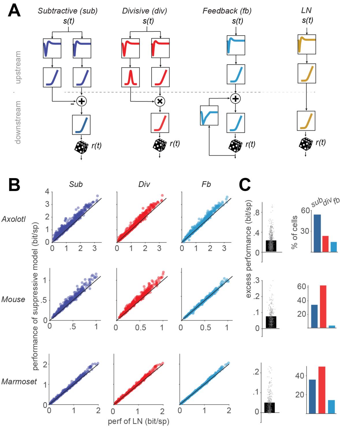
Figure 1. Schematic of the models and their overall performance. A) Structure of the three suppressive models used in our study with subtractive, divisive, and feedback suppression and of the LN model. B) Comparison of the performance of each model, measured as the information provided by each spike, to the performance of the LN model. Each data point represents one cell. C) Left: The excess performance (performance of suppressive model minus LN-model performance) of the best performing suppressive model, determined for each cell. Right: the percentage of cells for which each of the suppressive models outperformed all the other models.
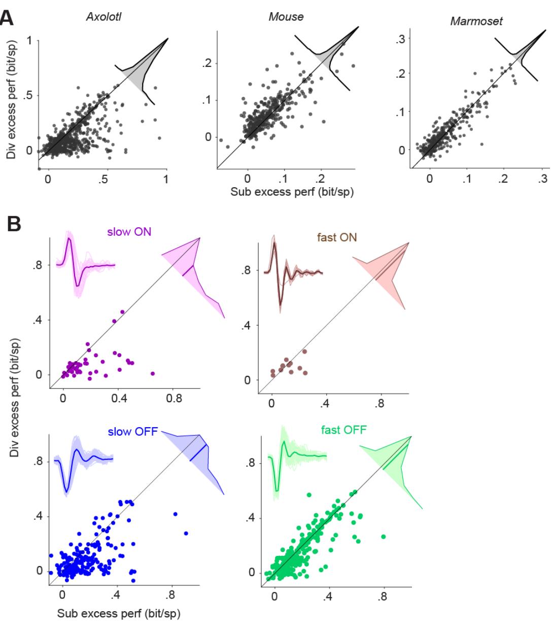
Figure 2. Comparison of the excess performance of the subtractive and the divisive model. A) Scatter plot of the excess performance of the subtractive model vs. the divisive model across each species. Each data point is a cell. Inset: The distribution of the performance difference between the subtractive and the divisive model. B) Same as A, but for slow/fast and ON/OFF sub-groups of the cells recorded from axolotl retina. Insets: The filters of the LN model of all cells within the subgroup (thin lines) and their average (thick line).
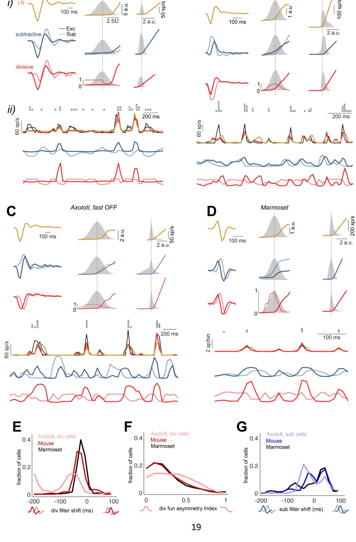
Figure 3. Model fits and response predictions sample cells from each investigated species. Ai) Excitatory and suppressive filters (left), upstream nonlinear functions (middle), overlapped with the distributed of its input which was the accompanying filtered stimulus, and output rectifier (right), overlapped with the distribution of its input which was the overall potential from the upstream, for the LN, the subtractive, and the divisive model. The feedback model was omitted, due to its lower performance, but the LN model was included for comparison. Aii) For a subsection of test-trial period: 1st row: spike counts per stimulus time bin for a sample test trial. 2nd row: the cell’s firing rate (black) and the predictions of three models. 3rd row: the output of the excitatory (solid line) and suppressive (dashed line) upstream branches for the subtractive model. 4th row: same as the 3rd row but for the divisive model. B, C, D) Same as A for other sample cells. E) The shift in the suppressive filter of the divisive model, compared to the excitatory filter, calculated in a similar fashion as E. F) The asymmetry index for the suppressive nonlinear function of the divisive model. The index was calculated as the absolute difference between the sum of the function values over negative and positive inputs, divided by the total sum of the function values. G) The shift in the suppressive filter of the subtractive model, relative to the excitatory filter across all cells. To calculate the shift for each cell, the cross-correlogram of the excitatory and suppressive filters were calculated, then the shift in the peak of the cross-correlogram was found.
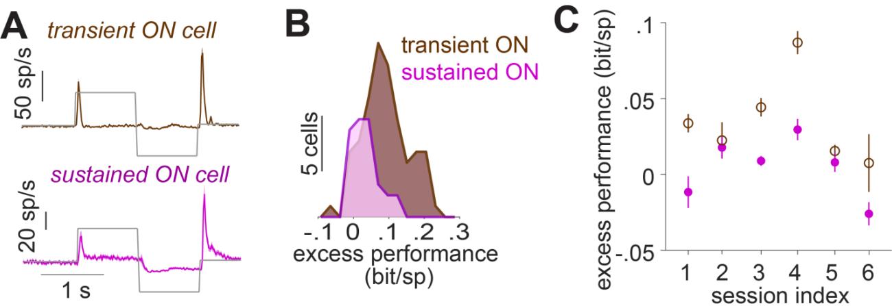
Figure 4. A) The responses of marmoset cells to a step stimulus for transient-ON and sustained-ON cells, averaged across all cells in a sample session (session index = 3). B) Distributions of the excess performance of the best-performing model, across transient and sustained ON cells for the same sample session. C) Mean and standard error of the excess performance for transient- and sustained-ON cells in each recording session.
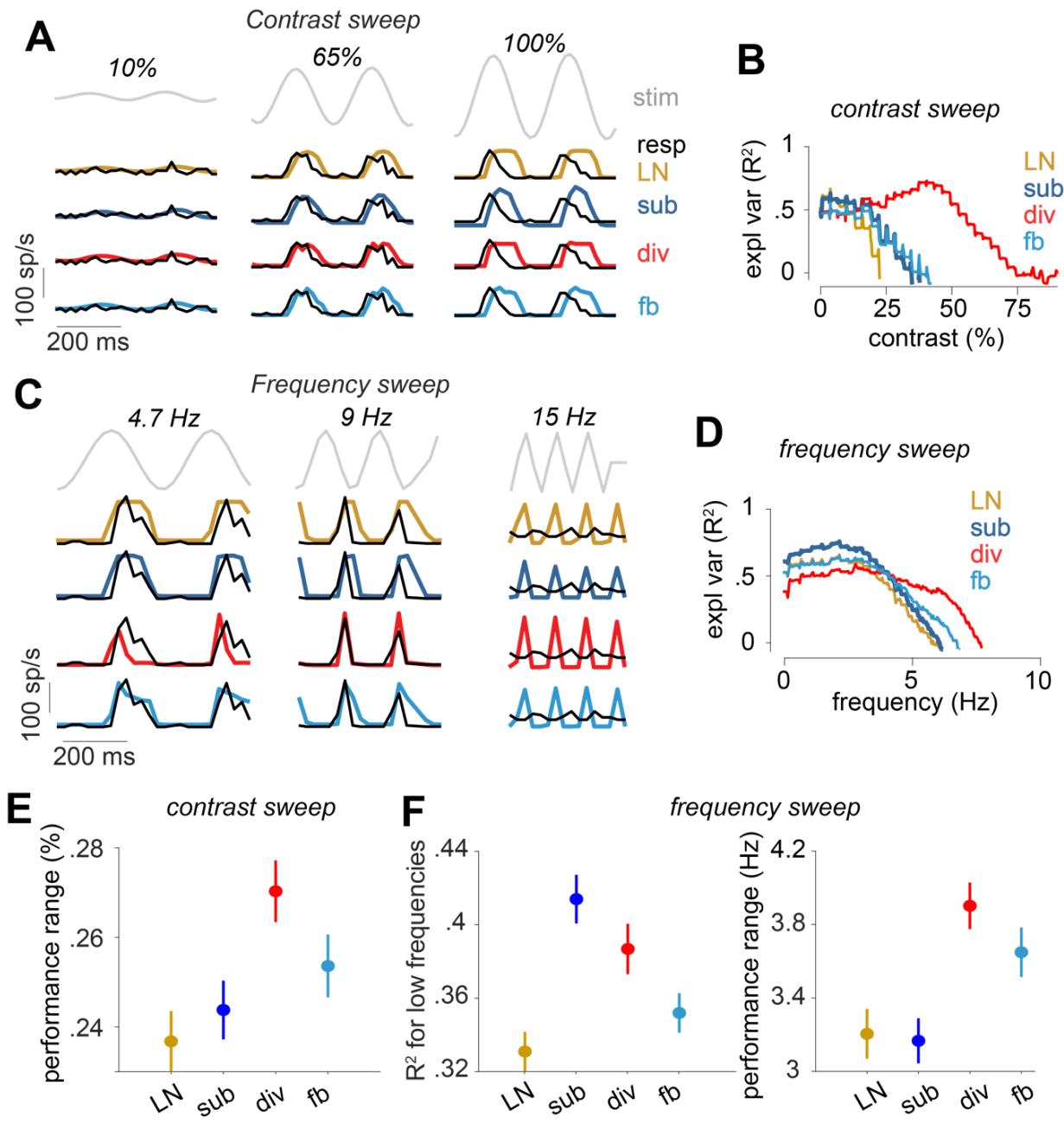
Figure 5 Evaluation of the models on responses to contrast and frequency sweeps for marmoset cells. A) Part of the contrast-sweep stimulus together with the response of a sample cell and the model predictions. Three sections of the contrast sweep are shown. The complete range of the stimulus, the cell response and the model predictions are shown in Fig. S6 B) Explained variance for the models for the cell in A, computed within a 150 ms sliding window. For each model, only the R2 > 0 range of values is shown. C) and D) Same as A and B, but for the frequency sweep instead of the contrast sweep for a different sample cell. E) The range of the contrasts for which each model had R2 > 0 (mean and standard error over cells). F) Left: The R2 of each model for the first 167 ms of the frequency sweep (10 stimulus frames) in the frequency sweep (mean and standard error over cells). Right: The frequency range for which each model had R2>0 (mean and standard error over cells).
¶ Methods
¶ Electrophysiology
All the experiments and procedures conformed to national and institutional guidelines and were approved by the institutional animal care committee of the University Medical Center Göttingen (protocol number T11/35).
The axolotl recordings were performed using 60-electrode perforated multielectrode arrays (MultiChannel Systems, Reutlingen, Germany; 30 µm electrode diameter and 100 µm minimum electrode spacing) as described previously32,33. The eyes were enucleated after 1 hour of darkadaptation and the retina was mounted over a 1.5-2 mm hole on a nitrocellulose filter membrane with the RGC-side down. During the experiment, the retina was perfused constantly with oxygenated (95% O2 and 5% CO2) Ringer’s medium (110 mM NaCl, 2.5 mM KCl, 1 mM CaCl2, 1.6 mM MgCl2, 22 mM NaHCO3, 10 mM D-Glucose monohydrate) at room temperature (~22°C). The mouse recordings were done with 252-electrode arrays (MultiChannel Systems, Reutlingen, Germany; 30 µm electrode diameter, and 100 or 200 µm minimum electrode spacing) as described previously34,35. The mice (aged 8-13 weeks, of either sex) were dark-adapted for at least 1 hour and subsequently euthanized by cervical dislocation. The eyes were removed quickly and transferred to a chamber with oxygenated (95% O2 and 5% CO2) Ames’ medium (Sigma-Aldrich, Munich, Germany), buffered with 22 mM NaHCO3 (to maintain pH of 7.4) and supplemented with 6 mM D-glucose. The eyes were dissected, and the cornea, lens, and vitreous humor were carefully removed. The retina was isolated from the pigmented epithelium and transferred to a multielectrode array. The temperature of the recording chamber was kept constant around 32–34°C, using an inline heater (PH01, MultiChannel Systems, Reutlingen, Germany) and a heating element below the array (controlled by TCX-Control 1.3.4, MultiChannel Systems), while the retina was perfused continuously with oxygenated Ames’ medium (4–5 ml/min).
For both axolotl and mouse recordings, the activity of the ganglion cells was amplified, band-pass filtered (300 Hz to 5 kHz), and recorded digitally at 25 kHz (60 MEAs) or 10 kHz (252 MEAs) using the MC-Rack software (Version 4.6.2, MultiChannel Systems). The spikes were extracted from the recorded voltage traces with a custom-made spike-sorting program based on a Gaussian mixture model and an expectation-maximization algorithm36.
The recordings from marmoset retina were performed as described previously37. Briefly, retinas were obtained from animals used by other researchers, in accordance with national and institutional guidelines and as approved by the institutional animal care committee of the German Primate Center and by the responsible regional government office (Niedersächsisches Landesamt für Verbraucherschutz und Lebensmittelsicherheit, permit number 33.19-42502-04-17/2496). Eyes were quickly enucleated and dissected to allow direct supply to the retina of oxygenated (95% O2 and 5% CO2) Ames’ medium (Sigma- Aldrich, Munich, Germany), supplemented with 6 mM D-glucose, and buffered with 22 mM NaHCO3 to maintain a pH of 7.4. Retinas were then dark-adapted for 1-2 hours. For each recording, a small peripheral retina piece, with pigment epithelium removed, was placed onto a 4096-channel CMOS-based microelectrode array (21 µm electrode size and 42 µm pitch; 3Brain AG). The retina piece was mounted with the RGC-side down, covered with a piece of translucent polyester filter membrane (Pieper Filter #PE0104700; 0.1 µm pores), and weighted down with a metal ring. During the recording, the retina was perfused with the oxygenated Ames’ medium (4-5 ml/min), and the temperature of the recording chamber was kept constant around 33°C in the same way as for the mouse recordings. Spike extraction and sorting were performed by HerdingSpikes2 (github.com/mhhennig/HS2). In short, spiking events were detected independently at each electrode using a fixed threshold, then simultaneous events in neighboring electrodes were triangulated to identify the location and shape of the spike. Finally, events were clustered into units, using a mean-shift algorithm, based on the location and first two principal components of the spike waveform38,39.
All retina preparations were performed under infrared illumination with a stereomicroscope equipped with night-vision goggles.
¶ Visual stimulation
Visual stimuli for all recordings were generated and controlled by a custom-made software written in C++ and using the OpenGL library. For both axolotl and marmoset recordings, the stimuli were presented on a monochromatic gamma-corrected white OLED monitor (eMagin, 800x600 pixels, 60 Hz refresh rate). For the mouse recordings, the stimuli were displayed via modified version of DLP Lightcrafter projectors (evaluation module (EVM), 864 × 480 pixels, 60 Hz refresh rate, Texas Instruments Company, Dallas, USA), with the blue LED replaced by a UV LED (emission peak at 365 nm), as described previously35.
The white-noise stimulus was obtained by drawing new screen intensities randomly from a normal distribution at either 30 Hz (axolotl) or 60 Hz (mouse and marmoset). The normal distribution of screen intensities was centered at half of the maximum intensity of the display and had a standard deviation of 30% of the mean light intensity. In the recordings from axolotl and mouse retinas, a fixed white-noise sequence of 300 intensity values (“frozen noise”) was repeatedly inserted after every 900 intensity values of non-repeating white noise.
The contrast-step stimulus, the contrast sweep, and the frequency sweep were presented consecutively, in a combo called the chirp stimulus16. In each trial of the chirp stimulus, following 120 frames of darkness (0% contrast), ON and OFF stimuli (100% and 0% contrast, respectively) were presented for 60 frames each. After another 60 frames of darkness, the sinusoidal frequency sweep was presented, starting at 0 Hz and ending at 15 Hz for a duration of 480 frames, fluctuation around the mean stimulus intensity with peak light levels at 0 and 100% contrast. After another 60 black frames, the sinusoidal contrast sweep was presented, starting at 0% and ending at 100% at frequency of 4 Hz for a duration of 480 frames. At the end, there were another 60 black frames. The chirp stimulus was repeated for 15 trials. The step part of the chirp stimulus was used for classifying cells into transient and sustained cells. The frequency and contrast sweeps were used for evaluating the generalization of the models to a range of stimulus frequencies and contrasts.
¶ Model construction and training
Each model contains one (for the feedback and the LN model) or two branches (for the subtractive and the divisive models) that represent upstream computation, followed by an output rectifier and a spike generator. Each upstream branch consists of a stimulus filter followed by a nonlinear function. The feedback model’s feedback loop consists of a filter that is applied to the recent history of spiking activity with no nonlinear function (Fig. 1A of the manuscript).
To maximize the consistency in implementation and training, we combined all four models in one master structure (Fig. S1).
Each filter as well as each upstream function was parameterized with a set of basis functions 11 (Fig. S7A shows the basis-functions for the filters and Fig. S7B shows the basis-functions for the nonlinearities).
The output rectifier was described as a “softplus” function:
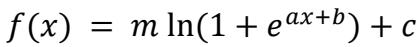
with a, b, c, and m representing free parameters.
In the unified structure, only one model component, i.e. a filter, an upstream function or the rectifier function, was trained at a time. Therefore, we can describe the output of this structure as the expansion of the branch that is under training using the basis functions while describing the rest of the model as a minimum set of variables as below:
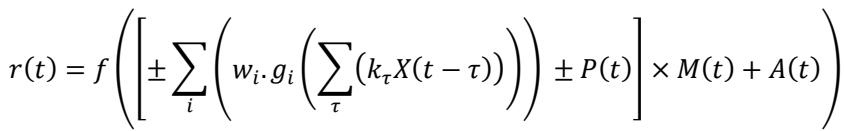
in which 𝑘𝜏 and 𝑤𝑖 are the weights for the basis functions for the filter and function under training, 𝑓 is the output rectifier, and 𝑔𝑖 are the pre-specified basis functions of the nonlinearities. For training each branch of each model, variables 𝑋, 𝑃, 𝑀 and 𝐴 were define from Table 1. This table shows, for example, that when the excitatory branch of the subtractive model was being updated, it was represented as the weighted sum term in the formula above, while the suppressive branch was represented by variable 𝑃 and vice versa. Similarly, for the divisive model, when the excitatory branch was being updated, the suppressive branch was represented by M and vice versa. Note that M is multiplicative in the formula, but acts as suppression, because the output of the suppressive branch is constrained to be in the range of zero to unity, owing to the constraint on its nonlinear function.
Table 1 Assignment of the variables to derive each model from the unified structure.
| Model | Components | X | P | M | A |
|---|---|---|---|---|---|
| Subtractive | exc (Excitatory) | stim | sup output | 1 | 0 |
| sup (Suppressive) | stim | exc output | 1 | 0 | |
| Divisive | exc | stim | 0 | 0 | sup output |
| sup | stim | 0 | 0 | exc output | |
| Feedback | exc | stim | 0 | 1 | feedback output |
| sup | spikes | 0 | 1 | exc output | |
| LN | exc | stim | 0 | 1 | 0 |
The under-the-training branch was updated using a block-coordinate ascent algorithm in which 𝑘𝜏 are updated to maximize the likelihood function, while wi were constant and vice versa. The components of the model were trained in this order: upstream excitatory, upstream suppressive (for subtractive and divisive models), the feedback loop (for the feedback model) and the output rectifier.
The objective function was −𝐿𝐿, negative of the log of the likelihood function, and was calculated as the log of the probability that the number of spikes at the time bin t was drawn from a Poisson distribution with the mean value of 𝑟(𝑡). In each step of the algorithm, we used function fmincon in Matlab® to take 10 steps per model component toward minimizing the objective function and we repeatedly trained all model components t either 100 times or until the change in the objective function was smaller than 0.01%. In fmincon, we used ‘trust region reflective’ algorithm. The constraints on the wi were applied using the sequential quadratic programming algorithm. The derivative of the objective function was provided to fmincon by calculating the derivative of −𝐿𝐿 to either 𝑤𝑖 or 𝑘𝜏. The constrains for each variable were chosen from table 2.
Table 2 The optimization constraint for the set of variables of each model component
| Model | Exc filter | Exc function | Sup filter | Sup function |
|---|---|---|---|---|
| Subtractive | Norm = 1 tail = 0 |
Monotonically increasing Lower bound = 1E⁻¹⁶ |
Norm = 1 tail = 0 |
Monotonically increasing Lower bound = 1E⁻¹⁶ |
| Divisive | Norm = 1 tail = 0 |
Monotonically increasing Lower bound = 1E⁻¹⁶ |
Norm = 1 tail = 0 |
Monotonically increasing for input < 0 & decreasing for input > 0 Scaled to [1E⁻¹⁶, 1] |
| Feedback | Norm = 1 tail = 0 |
Monotonically increasing Lower bound = 1E⁻¹⁶ |
tail = 0 | - |
| LN | Norm = 1 tail = 0 |
Monotonically increasing Lower bound = 1E⁻¹⁶ |
- | - |
* The tail of the filter was the average of the values of the last 5 time-bins.
To reduce the risk of finding non-optimal solutions corresponding to local minima of the objective function, the training was repeated 5 times with different initializations that were guided by simple spike-triggered analyses. We then selected the solution for which the value of the objective function (negative log-likelihood) for the training data was the lowest. The initial values were selected from the spike-triggered average, the most relevant stimulus features extracted from a spike-triggered-covariance analysis40,41, pre-defined deterministic functions and Gaussian noise as in table 3 (when different initial values were used for each model, they follow the format of sub / div / fb / LN) where STA was the spike-triggered average, STC1 and STCN where the first and the last principal components of the spike-triggered covariance, Wmono was the softplus function, as defined above, with a = 10, b,c = 0 and m = 0.1, Wbi was an inverted bell-shaped function between 0 and 1. Gaussian noise with a mean of 0 and standard deviation of 0.1 was added to Wmono and Wbi, each time that they were used.
Table 3 Initial values for 5 training iterations
| Iteration | Exc filter | Exc function | Sup filter | Sup function |
|---|---|---|---|---|
| 1 | STA | Wₘₒₙₒ | STC₁/STC₁/0/- | Wₘₒₙₒ / Wᵦᵢ / - / - |
| 2 | STA | Wₘₒₙₒ / Wᵦᵢ / Wₘₒₙₒ / Wᵦᵢ | STC₅/STC₅/0/- | Wₘₒₙₒ / Wᵦᵢ / - / - |
| 3 | STC₁ | Wₘₒₙₒ | STC₅/STC₅/0/- | Wₘₒₙₒ / Wᵦᵢ / - / - |
| 4 | STC₅ | Wₘₒₙₒ / Wᵦᵢ / Wₘₒₙₒ / Wᵦᵢ | STC₁/STC₁/0/- | Wₘₒₙₒ / Wᵦᵢ / - / - |
| 5 | N(0,1) | Wₘₒₙₒ | N(0,1) | Wₘₒₙₒ / Wᵦᵢ / - / - |
For all models and iterations, the initial value of the output rectifier was 10∗ln(1+𝑒0.1𝑥).
¶ Evaluation and cross-validation
The best solution of each model for each cell was evaluated on both training and testing data. For the feedback model, the performance was averaged across 100 evaluations, each with spike counts obtained stochastically according to a Poisson distribution with rate given by the model’s output. When frozen noise data was available (axolotl and mouse data), it was held out as the test data. Otherwise (marmoset data), 5 s of data were taken from every 25 s as pseudo-trials for testing.
¶ Selection of units
After sorting the recorded spikes into single units, a subset of units was selected for modeling based on multiple criteria: 1. The average firing rate of the unit under the white-noise stimulus was required to be larger than 2 Hz for axolotl and larger than 5 Hz for mouse and marmoset. 2. The explainable variance was required to be larger than 0.5. The explainable variance was calculated by dividing the responses of a cell to the set of frozen noise stimuli to two subsets, averaging the cell response within each subset, then calculating the explained variance of the response average across the first subset by the response average of the second subset. The explainable variance was calculated as the average of this explained variance, across 20 randomly divided subsets. 3. The difference between the average firing rate in the early (< 30% of the total recording time) and late (> 70% of the total recording time) part of the recording under the white-noise stimulus was required to be less than 50% of the overall average firing rate. 4. The unit was required to not correspond to an ON-OFF cell, i.e., it should not respond to both light increments and light decrements. ON-OFF cells were detected by the U-shape nonlinear function of the LN model: The function was divided into the left (input < 0) and the right (input > 0) parts, then a line was fitted to the left (slope = sL) and another line was fitted to the right parts (slope = sR). A cell was classified as ON-OFF, if sL / (|sL| + |sR|) < -0.2. 5. Performance on the test data was required to be at least 60% of the performance on the training data for all four models to reduce the effects of overfitting.
Repeated units were detected and removed, based on the similarity between their responses to white-noise stimuli. To that end, the firing rate of each cell was binned according to stimulus frames, then the cross-correlation between the binned firing rates was calculated for all pairs of cells within a simultaneously recorded population. The strength of response correlation was then calculated as the value of the center of the cross-correlogram (lag = 0). Next, a graph of the simultaneously recorded cells was made with one node for each cell and one edge between two nodes if the response correlation between two cells was > 0.3. Repeated cells were detected by finding cliques within this graph. Within each group of repeated cells, all except the one with the maximum explainable variance were removed.
¶ Statistical analysis
Two-sided Wilcoxon signed-rank test was used, except where another test was indicated. When multiple groups of data were compared, false discovery rate (FDR) correction for multiple comparisons15 was used to correct the p-values.
¶ Supplemental figures
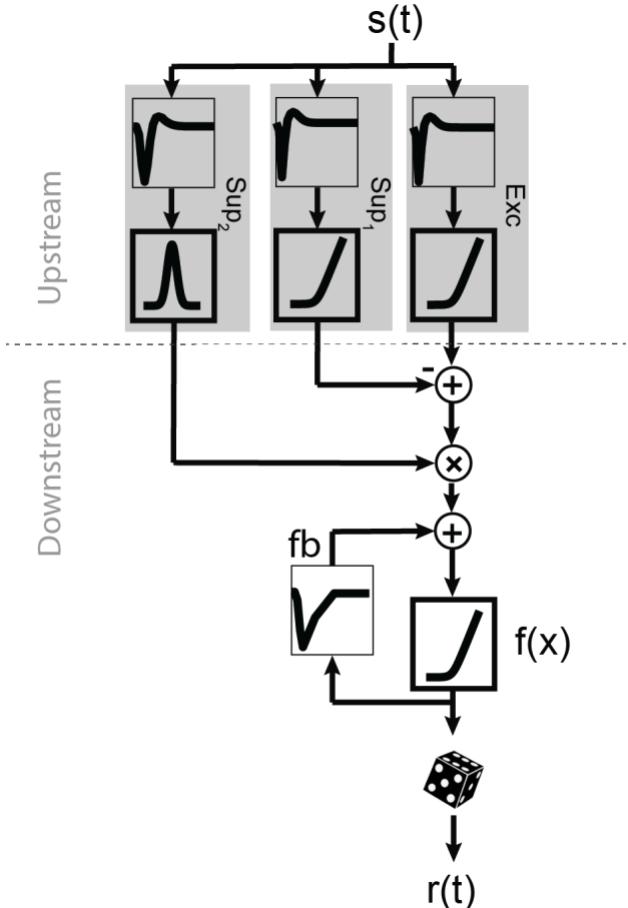
Figure S1 The unified model structure that incorporates all components in the models in Fig. 1A. The filter components are shown in thin frames and the nonlinearities in thick frames. Exc upstream branch represents the excitation, Sup1 represents the subtractive suppression, and Sup2 represents the divisive suppression. The feedback (fb) was added to the downstream part of the model.
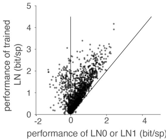
Figure S2 Comparing the performance of our trained LN model to the performance of an LN model which uses the STA as the filter and the associated spike histogram as the nonlinear function (LN0) or the first principal component of STC as the filter and the associated spike histogram as the nonlinear function (LN1). 12 cells for which the performances of LN0 and LN1 where < -2 bit/s where omitted.
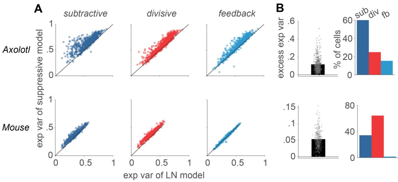
Figure S3 Same as Fig. 1B-C, but for Poisson explained variability. A) Comparison of the Poisson explained variability of each model to the performance of the LN model. Each data point represents one cell. B) Left: The excess explained variability (exp var of suppressive model minus exp var of the LNmodel) of the best performing suppressive model, determined for each cell. Right: the percentage of cells for which each of the explained variability of the suppressive models was higher than all the other models.
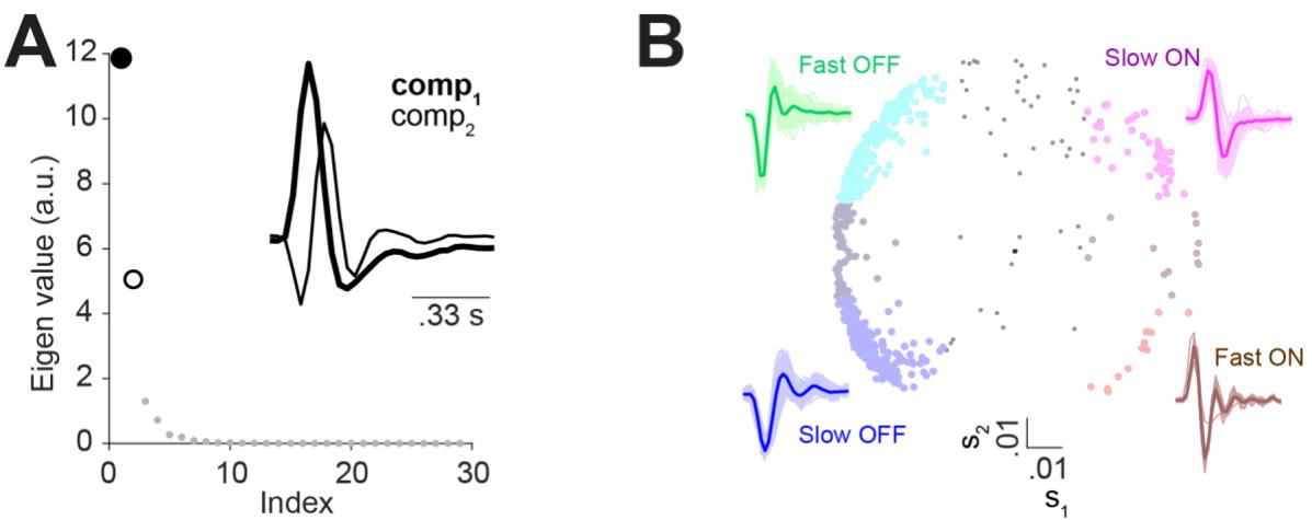
Figure S4 Principal component analysis of the excitatory filter shapes to separate cells recorded from axolotl retina into functional classes. A) The eigenvalues associated with 30 principal components of the filter of the LN model. Inset: The first and the second principal components, which were used for classification. B) Center: All analyzed axolotl cells in the space of s1, the scores for the first principal component and s2, the score for the second principal component. To determine the classes, the scores for each cell were compared to 0.02 for the 1st and 0.5 SD = 0.02 for the 2nd component: for slow ON cells (n = 48) s1 > 0.02 and s2 > 0.02, for fast ON cells (n = 13) s1 > 0.02 and s2 < -0.02, for slow OFF cells (n = 195) s1 < -0.02 and s2 < -0.02 and for the fast OFF cells (n = 208) s1 < -0.02 and s2 > 0.2. 143 cells stayed unclassified due to not passing either of the thresholds. Surround: LN-model filters (thin lines) for each of the identified groups, together with their average (thick line).
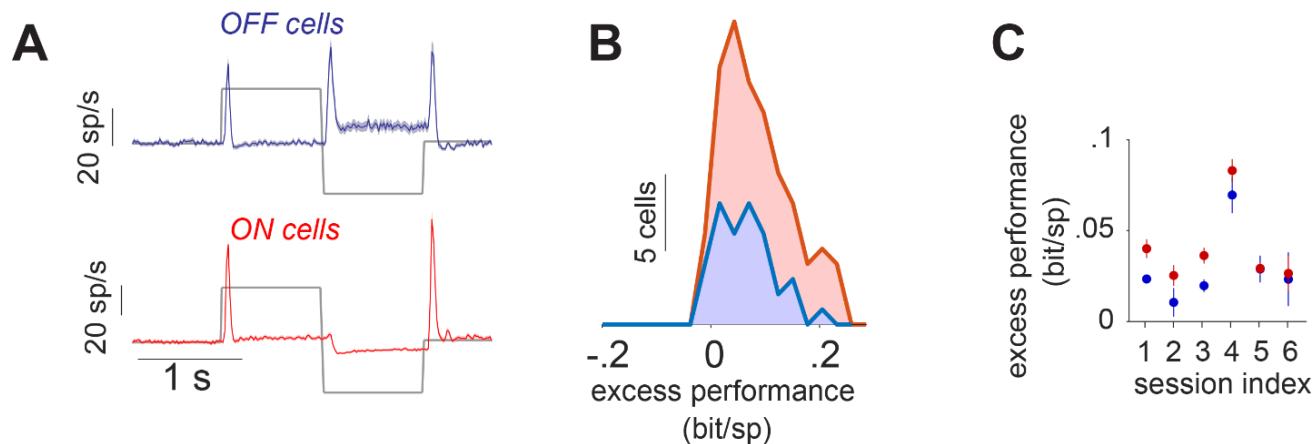
Figure S5 The performance of the best performing model for marmoset ON and OFF cells under stimulation with steps in light intensity. The analysis was performed in a similar fashion as in Fig. 4. A) Classification to ON and OFF based on the cells’ response to a step stimulus. The average of the responses within each class is shown for a sample session. B) Distributions of the excess performance of the best performing model, across On and OFF cells for a sample session. C) The performance of the best performing model for the cells within each recording session.
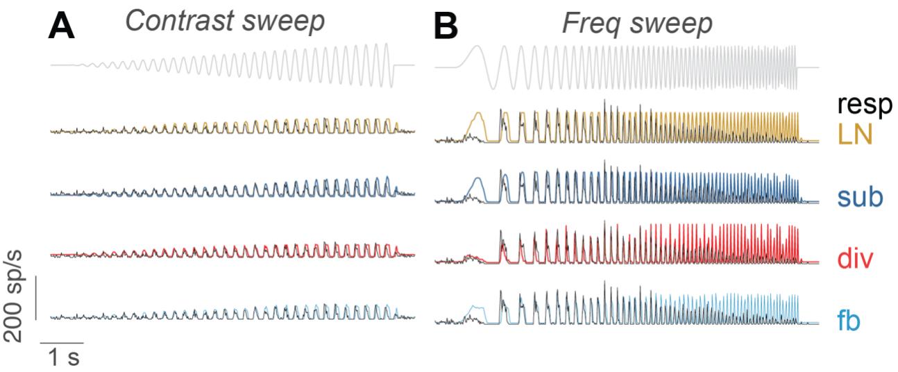
Figure S6 The responses of sample cells in Fig. 5A-D and the model predictions for the entire ranges of the contrast sweep and the frequency sweep. A) The cell in figure 5A-B. B) The cell in figure 5C-D.
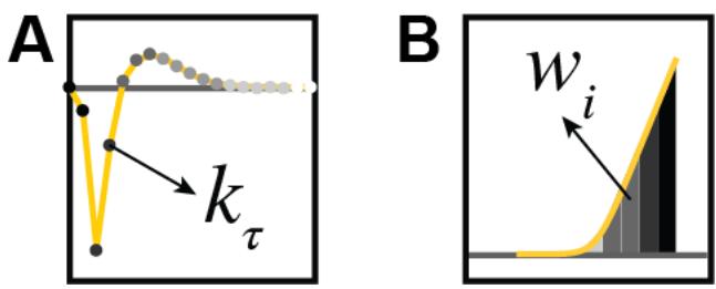
Figure S7 The basis-functions for filters as well as the upstream output functions. A) Each basis function for the filters (the gray points) was one time-bin (stimulus frame). 30 basis functions were used for axolotl and mouse and 15 basis functions for marmoset, due to the faster dynamics of the responses in marmoset RGCs, compared to the other species. 20 basis functions were used for the feedback filter of all cells. B) Each basis function for the output functions was a tent-shaped function (gray tents). All bases together provide a piece-wise linear estimation of the function. 15 basis functions, covering [-3,3], were used.